About Insights - Parallel, High-dimensional Self-organizing Knowledge Mining from Noisy Data

▲

Insights Application.

Modeling and Forecasting a National Economy as Interdependent System.

In economic and financial research analysis of economic systems and multi-step ex ante forecasting of key economic parameters are gaining importance. The purpose of such studies is to create preconditions appropriated for expected future developments and to find the laws and factors of influence causing these developments. This example demonstrates the power and results of self-organizing modeling and identification of the interdependence structure of 14 key parameters of the German national economy. This system model (system of equations) developed by Insights in minutes from historical data is then used to autonomously forecast several uncertainty-driven scenarios of all economic parameters five years ahead up to the year 2021 and is compared to corresponding forecasts of the International Monetary Fund (IMF).

Modeling

Given are data of 14 economic parameters of the German national economy of the years 1980 to 2016 (N = 37) as provided by the IMF (World Economic and Financial Surveys, World Economic Outlook Database, 2016), which can be a priori divided into endogenous or state variables x and exogenous variables u:

x₁: Gross domestic product, constant prices [Billion EUR]
x₂: Gross domestic product, deflator
x₃: Gross domestic product per capita, constant prices [Billion EUR]
x₄: Output gap in percent of potential GDP [%GDP]
x₅: Gross domestic product based on purchasing-power-parity (PPP) per capita GDP [USD]
x₆: Gross domestic product based on purchasing-power-parity (PPP) share of world total [%]
x₇: Total investment [%GDP]
x₈: Gross national savings [%GDP]
x₉: Inflation, average consumer prices
x₁₀: Volume of imports of goods and services [%change]
x₁₂: Unemployment rate [%]
x₁₃: Employment [Mill]
x₁₄: Population [Mill]

u₁₁: Volume of exports of goods and services [%change]

Using a maximum time lag of five for each of the 14 economic system parameters sums up to 84 inputs for self-organizing a linear system of 13 difference equations (14 variables minus one exogenous variable, u₁₁), and the modeling task is defined mathematically by:

It is important to note that for linear dynamic systems also non-lagged inputs of the endogenous variables can be used for modeling since Insights takes care that only mathematically conflict-free systems will be developed to allow their application for ex ante forecasting. Mathematically conflict-free here means that the system contains no closed dependencies between the non-lagged inputs. Graphically, this means that there is no closed loop of dependencies between non-lagged inputs. For example, the system

x_1,t = f₁(x_3,t, .)
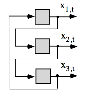
x_2,t = f₂(x_1,t, .)
x_3,t = f₃(x_2,t, .)

is not free of conflicts, because each variable x_i,t is self-depending via the system structure at a time t. Such conflicted systems cannot be used for ex ante forecasting (fig. 1).

closed loop of linear system of equations

Fig. 1: Closed loop between non-lagged variables reflecting self-references.

Results

As a result of noise and uncertainty in the input data for modeling Insights generally provides not only one best but a number of qualitatively and quantitatively comparable models according to model accuracy. Therefore, a set of system models is developed implicitly. One self-organized system of equations is given below and the corresponding identified interdependence structure of the autonomous system is shown in figure 2.

x₁(t) = 0.08094716x₃(t) + 24.29554x₁₄(t) - 1961.904
x₂(t) = 0.4980568x₉(t-1) + 2.011354x₁₃(t-1) + 2.958109x₁₄(t-1) - 262.6105
x₃(t) = 296.7671x₄(t) + 144.5323x₉(t) + 129.4768x₉(t-5) + 7295.092
x₄(t) = 0.00136263x₅(t) - 0.0006133768x₅(t-1) - 0.0007974957x₅(t-3) - 0.9018034x₁₂(t) - 0.5752203x₁₃(t) +
+ 1.256526x₁₄(t-1) - 0.5413245x₁₄(t-3) - 32.00273
x₅(t) = 7.804878x₁(t-1) - 5735.344x₆(t-1) + 1207.645x₁₃(t) - 3110.653
...
x₁₄(t) = 0.03410858x₁(t-1) - 0.001863582x₃(t-1) + 0.1238598x₄(t-2) - 0.0003100284x₅(t-1) +
+ 0.03877476u₁₁(t) - 0.1946272x₁₄(t-4) + 80.66718

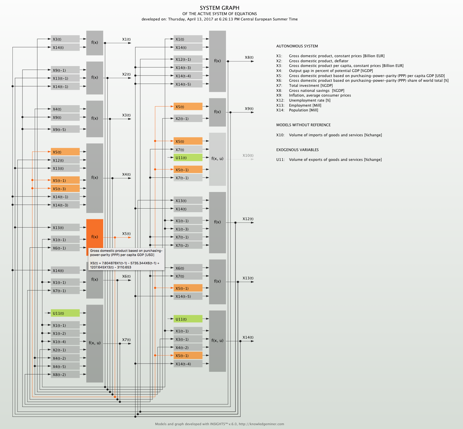
Fig. 2: System graph of the self-organized macroeconomic system of equations model.
This graph is interactive in Insights: When clicking on a gray model box the selected model gets highlighted and the references of this model are shown along with the model equation for quick overview.

Ex ante forecasting

Out of the set of developed system models Insights automatically generates a number of forecasts of all 13 endogenous system variables five years ahead to reflect model and forecasting uncertainty. This is similar to ensemble or scenario forecasting with a most likely forecast and a forecasting interval for each variable and forecasting step individually. These Insights forecasts are compared to the IMF forecasts, which, however, only provides a single, crisp forecast for each variable. Figures 3 to 6 show these forecasts for:

x₁ - Gross domestic product
x₇ - Total investment [%GDP]
x₈ - Gross national savings [%GDP] and
x₁₃ - Employment [Mill]

exemplarily.

Fig. 3: Ex ante forecast of state variable x₁ for the years 2017 to 2021 (green dots) along with forecasting uncertainty (gray area)
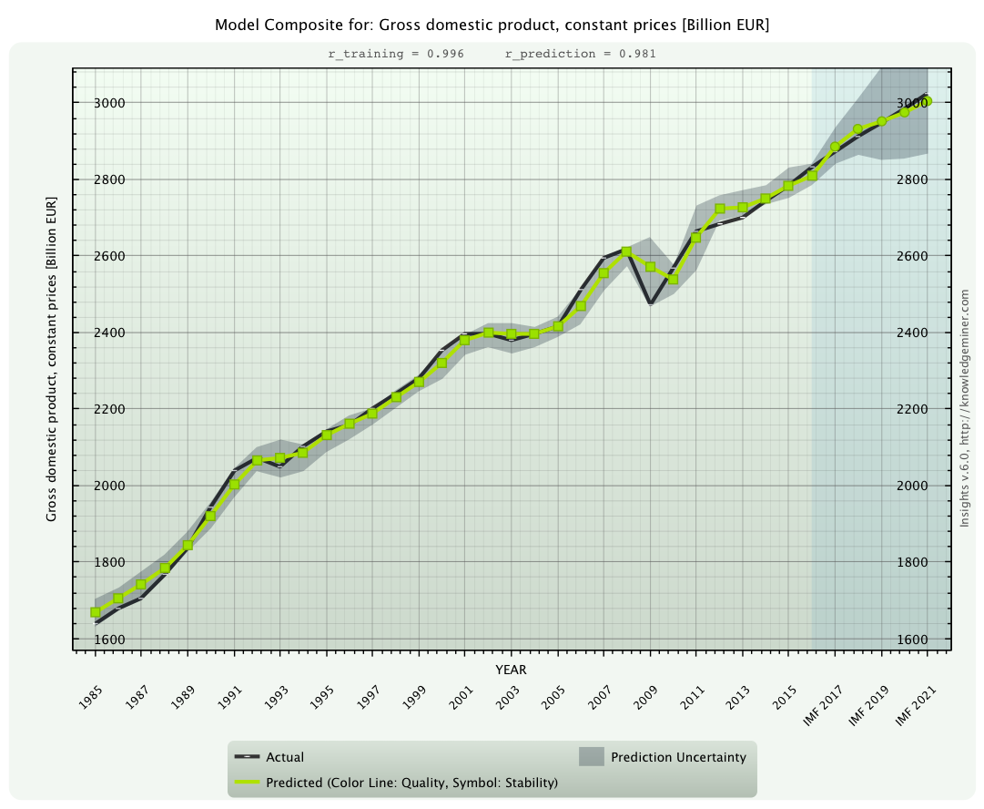
compared to the IMF forecast (black line).

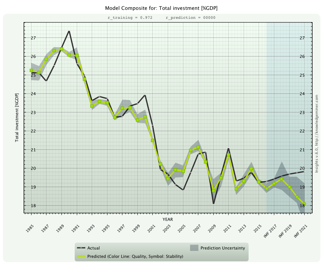
Fig. 4: Ex ante forecast of state variable x₇ for the years 2017 to 2021 (green dots) along with forecasting uncertainty (gray area)
compared to the IMF forecast (black line). A divergence of forecasted trends is clearly visible.

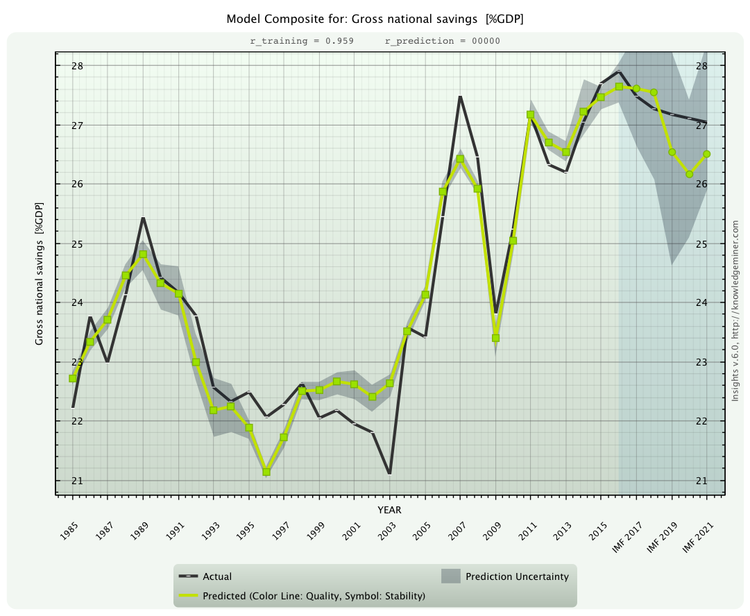
Fig. 5: Ex ante forecast of state variable x₈ for the years 2017 to 2021 (green dots) along with forecasting uncertainty (gray area)
compared to the IMF forecast (black line). This variable is connected with high uncertainty.

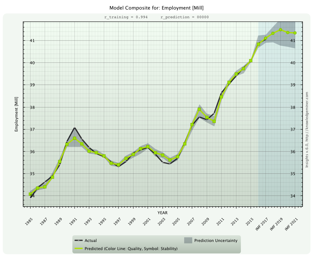
Fig. 6: Ex ante forecast of state variable x₁₃ for the years 2017 to 2021 (green dots) along with forecasting uncertainty (gray area).
For this key economic parameter the IMF provided no complete forecast.

Out-of-the-box 64-bit multi-core self-organizing data mining of Insights GMDH in Excel

Try out free.

Start using the value of your data today.