|
One original and powerful feature implemented in Insights is additional external evaluation of self-organized
linear and nonlinear analytic models. This document is about to show how this new model evaluation approach actively supports
answering the question if the obtained model reflects a valid, reliable, and in best case, causal relationship or if it's just
pretending model accuracy due to chance correlation, only. Also, a new model quality measure that takes into consideration the noise filtering power
of the modeling algorithm and model complexity is introduced: Descriptive Power.
The Problem
A key problem in data mining is final evaluation of developed models. This evaluation process is an important condition for
deployment of data mining models. By learning from a finite set of data, only, it is hardly possible to decide whether the
developed model reflects a valid relationship between input and output or if it's just a stochastic model with non-causal
correlations. Model evaluation needs, in addition to a properly working noise filtering procedure for avoiding overfitting
the learning data, some new external information to justify a model's quality, i.e., both its predictive and descriptive power.
Why
Let's have a look at this example: Based on an artificial data set of 2 outputs, 4 inputs, and 15 samples Insights
self-organizes an analytical model for each output variable, Y1 and Y2 (fig.1; red line: the model,
blue line (almost hidden): the original data).
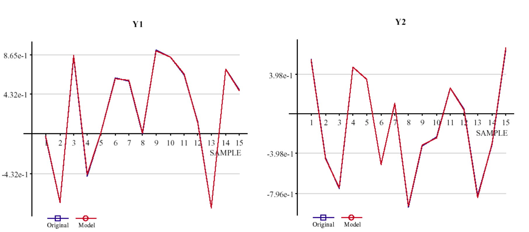
a) Model 1: Y1 = f1(x)
b) Model 2: Y2 = f2(x)
Fig. 1: Model graph of the two models M1 and M2.
For both models an accuracy (model fit on the learning data, R2,
for example, or a more complex criterion like PSE, AIC or BIC) of 99,9% is reported.
Concluding from this accuracy and from the graphs of fig. 1 there is no reason to not considering
both models as "true" models that reflect a causal relation between
output and input. Also, taking into account that KnowledgeMiner Insights, compared to the vast majority of data mining
tools, is implementing in its inductive self-organizing model synthesis a powerful noise filtering procedure,
already (see also "Self-Organizing Data Mining" book, section 3.2), this seems to underline the above assumption.
Now, assume that there is information that only one model
actually describes a causal relationship while the other model simply reflects
stochastic correlations. Although this information is given to you -
which is usually not the case in real-world - you cannot decide
from the available information which of the two models is the true model and which one
is the chance model. Only applying the models on some new data (which adds new information) will turn out
model M2 as the only valid model (fig. 2):
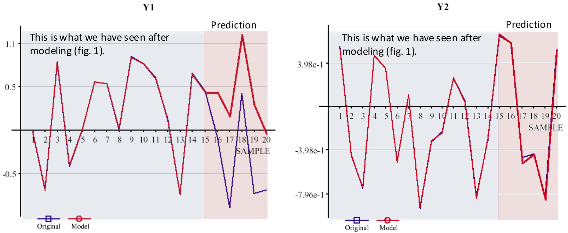
a) Model 1: invalid
b) Model 2: valid
Fig. 2: Prediction of models M1 and M2.
The Noise Filtering Behavior of an Algorithm
This example clearly shows that any "closeness-of-fit" measure is not sufficient to evaluate a model's
predictive and descriptive power. Recent research has shown that model evaluation requires a two-stage
validation approach (at least):
1. Level
Noise filtering to avoid overfitting the learning data based on external information (hypothesis testing) not
used for creating a model candidate (hypothesis) as an integrated part of the "Model Learning" process.
A corresponding tool that is used in Insights from the beginning within "Model Learning" is
leave-one-out cross-validation.
2. Level
A characteristic that describes the noise filtering behavior of the "Model Learning" process to justify
model quality based on external information not used in the first validation level. This noise-filtering
characteristic is implemented in Insights for the first time for linear and nonlinear analytical
models. This characteristic was obtained by running Monte Carlo simulations many times. In this way,
new and independent external knowledge is available that any model has to be adjusted with.
Figure 3 shows a detail of the characteristic for linear analytical models.
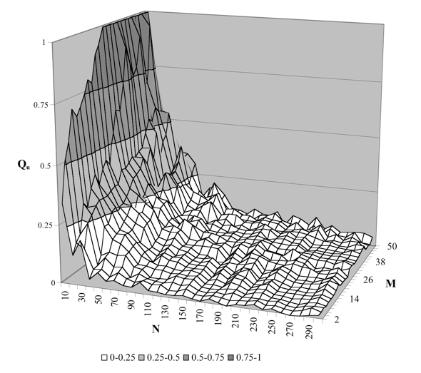
Fig. 3: Noise filtering characteristic
M: number of inputs; N: number of samples; Qu: virtual quality of a model
Qu = 1: noise filtering does not work at all; Qu = 0: ideal filtering
The reason for a second level validation is (1) that noise filtering implemented in level 1 is not
an ideal noise filter and thus is not working properly in every case (see this example) and (2) to get
a new model quality measure that is adjusted by the noise filtering power of the modeling algorithm.
The noise sensitivity characteristic expresses a pretending model quality
Qu that can be obtained when simply using a data set of M potential
inputs of N random samples. It is pretending model quality (accuracy), because, by definition,
there is not any causal relationship between stochastic variables a priori (true and
best model quality Q = 0, by definition), so - when using random samples -
any model of quality Q > 0 just pretends having that better quality and having the found
input-output relationship while we know that it actually does not exist. This means, given a
number of potential inputs M and a number of samples N, a threshold quality
Qu = f(N, M) is calculated by Insights that any model of quality Q must
exceed to be considered valid with respect to describing a relevant relationship between input and output.
Otherwise, a model of quality Q <= Qu is assumed invalid, since its
quality Q can also be obtained when simply using random variables, which means that this certain model's
quality does not significantly differ from a chance model. It has to be considered unreliable and invalid.
Descriptive Power
In addition to deciding if a model appears being valid or not, the
noise sensitivity characteristic is also a tool for calculating the
descriptive power of an input-output model, directly. It introduces a new model
quality measure, which is adjusted by model complexity and the algorithm's
noise sensitivity behavior and which, finally, is independent from the learning data set dimensions.
The Descriptive Power (DP) is defined as:
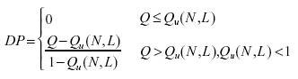
whith Q as the obtained accuracy of the evaluated model and Qu(N, L) as the reference
accuracy calculated from the number of samples N the model was created on and
the number of input variables L the model is actually composed of
(selected relevant inputs), with L <= M. This means that Descriptive Power is a chance-correlation-adjusted
quality measure, which is independent from the data set dimension used to develop the model.
Figure 4 shows an example of two models M1 and M2
which show the same accuracy Q = Q1 = Q2 but different
Descriptive Power since both models where obtained from data sets of different
sample lengths, and thus, different noise immunity of the modeling algorithm.
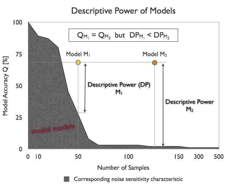
Fig. 4: Descriptive Power of two models.
Model Evaluation
The concept of an algorithm's noise sensitivity and Descriptive Power provide
additional external information required to check a model's validity with respect to
whether or not it distinguishes from a chance model and to which extent. Back to
the example at the top of this page this means that it is possible now to
identify suspect models right after modeling, automatically. For model M1 and
M2 the following evaluation results are reported in Insights:
MODEL EVALUATION: INVALID
The requested noise immunity could not be applied for the chosen sample length. Instead,
VERY POOR noise immunity was used for modeling, only. To get the requested noise immunity,
increase the number of samples to at least 21.
The model seems not reflecting a valid relationship. The likelihood that the data used for
modeling is actually random data with no existing input-output relationship is 33%.
Keep in mind, however, that the model was built using VERY POOR noise immunity. This makes
evaluation of the model more uncertain.
a) Report of Model 1 --> status: invalid
MODEL EVALUATION: VALID
The requested noise immunity could not be applied for the chosen sample length.
Instead, VERY POOR noise immunity was used for modeling, only. To get the requested
noise immunity, increase the number of samples to at least 21.
The model seems to establish a valid relationship. The Descriptive Power of the model relative to a chance
model is 42% for the actually used noise immunity.
a) Report of Model 2 --> status: valid
This means, the modeler (you) knows instantly that model 2 does well indeed with a Descriptive Power
of 42% while model 1 is seen invalid to 33%. Following the recommendation given in the report of model 1,
increasing the number of samples to 21, in a second modeling run KnowledgeMiner Insights now comes up with this report:
MODEL EVALUATION: INVALID
The model seems not reflecting a valid relationship. The likelihood that the data used for
modeling is actually random data with no existing input-output relationship is 67%.
The model was generated by self-organizing high-dimensional modeling.
Insights now reports an increased certainty of 67% that this model is just a chance model
and therefore has to be rejected. Interesting to note is also that this tiny modeling problem has
been identified as high-dimensional modeling task, which sounds strange, first. However, "high-dimensional"
has to be seen not only in absolute but also in relative terms: every modeling problem with a high number
of inputs-to-samples ratio is a high-dimensional modeling task, actually, with respect to model building
and validation and has to be handled as such.
Noise Immunity Levels in Insights
In KnowledgeMiner Insights, the noise immunity levels shown in figure 6 are
available to the user for building models of corresponding validity and reliability
by avoiding pretending model accuracy above the level it is assigned to.
If you choose a GOOD noise immunity for building a model, for example,
Insights will take care that at the end of modeling the resulting model
usually will not have a pretending accuracy above a value of 8% while for a POOR noise
immunity the pretending accuracy can have a value of up to 30%.
It is important to note that under certain conditions - especially if the
number of samples of the learning data set is small - validity and reliability
of a model on the one hand and model accuracy on the other hand may
become mutually exclusive goals: If I request increased model reliability model
accuracy may decrease and vice versa.
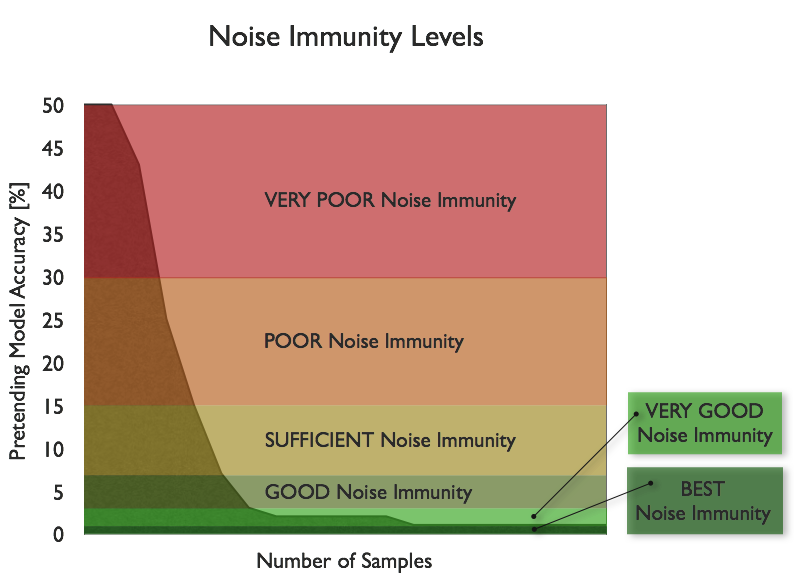
Fig. 6: Noise immunity levels for model self-organization used in INSIGHTS.
Summary
The two-stage model validation approach implemented in KnowledgeMiner Insights allows for the
first time in a data mining software to get active decision support in model evaluation
for minimizing the risk of false interpreting a model's quality and power and using invalid
models for prediction and classification tasks that in fact just reflect a chance correlation.
In combination with our original Live Prediction Validation technology, it gives you the highest
degree of reliability about your data mining models you get from software available on the market today.
|


 INSIGHTS